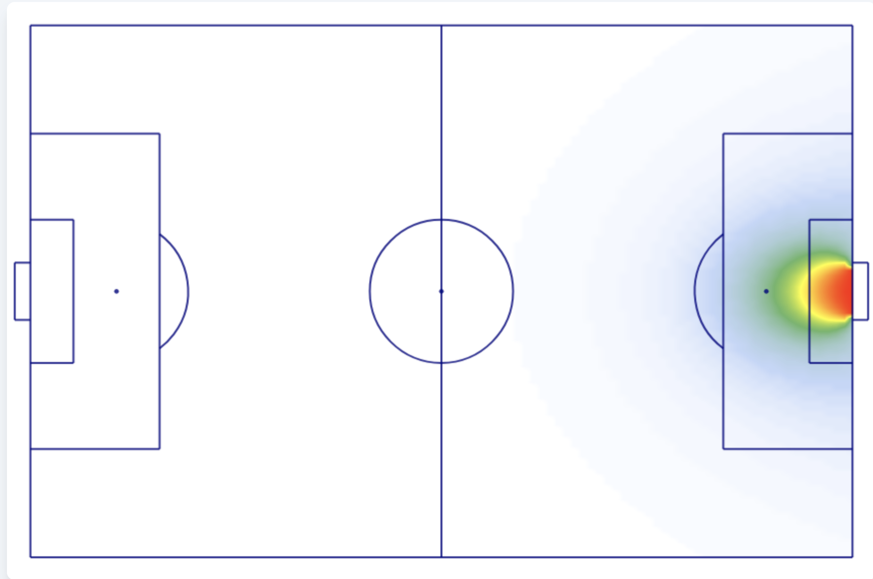
Custom Football xG Model & Interactive Plotter

This project is an interactive Expected Goals (xG) prediction and visualisation tool for football, built entirely from scratch. It lets you click on a pitch, specify the shot situation and type, and get an instant xG prediction back, all running directly in the browser with no server involved.

The underlying model family and much of the feature engineering philosophy carry the DNA of my final-year undergraduate dissertation from 2024, in which I achieved a first class grade for investigating whether xG models are genuinely predictive of future team performance across the top five European leagues. That research involved building and comparing logistic regression and random forest classifiers, scraping and processing a substantial dataset, and then evaluating how well those xG estimates could predict future team performance as features in regression and match outcome prediction models. The plotter is a ground-up rebuild of those ideas into something interactive and deployable, rather than an academic artefact that lives in a PDF and is never looked at again.

The Dissertation: Where It All Started

My dissertation asked a fairly fundamental question about the xG metric that many football analysts take for granted: does it actually predict future outcomes better than raw goal counts? The answer, perhaps unsurprisingly to anyone who has followed the analytics space, was broadly yes, though with some interesting nuance depending on which model variant you used and how far ahead you tried to predict.

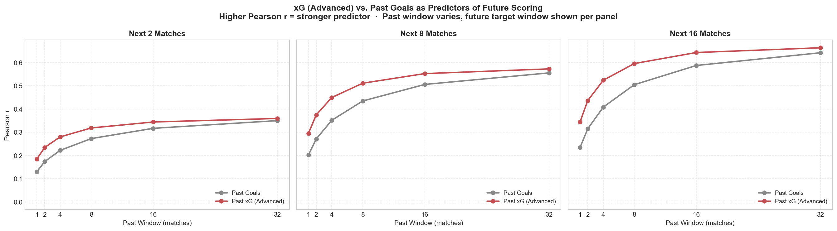
Figure: This analysis, building on ideas from my dissertation, compares how well past expected goals and past actual goals predict future player scoring performance. The Pearson correlation tracks predictive strength across varying match windows. Expected goals consistently outperform raw goal counts as a leading indicator of future attacking performance. This advantage is particularly pronounced in the short term and extends clearly through medium-term evaluations but the predictive power of expected goals and raw goals eventually converges over much longer time horizons.

To answer that question I needed to build xG models from scratch. The dissertation covered scraping historical shot data from Understat, cleaning and preprocessing it, engineering spatial features and training classifiers. Both logistic regression and random forest models were built and compared. Those xG estimates were then used as features in a separate set of predictive models, evaluated against standard regression metrics like MAE and MSE and tested in the context of match outcome prediction. That entire modelling workflow forms the academic foundation of what became the xG Plotter.

The key difference is intent. The dissertation was about the validity of xG as a predictive metric. The plotter is about making those models usable and visible, in a way that is actually enjoyable to interact with.

The Data Pipeline

The backend is a Python pipeline orchestrated by a single shell script, run_pipeline.sh, which runs five stages in sequence. Everything is configured from src/config.yaml, which specifies the target leagues and seasons.

Scraping

Shot data is scraped from Understat, covering the English Premier League, La Liga, the Bundesliga, Serie A and Ligue 1, for seasons spanning 2014 to 2025. That amounts to over half a million shots across roughly a decade of top-level football. Each record contains the normalised x/y coordinates of the shot, the game situation, the shot type and the outcome.

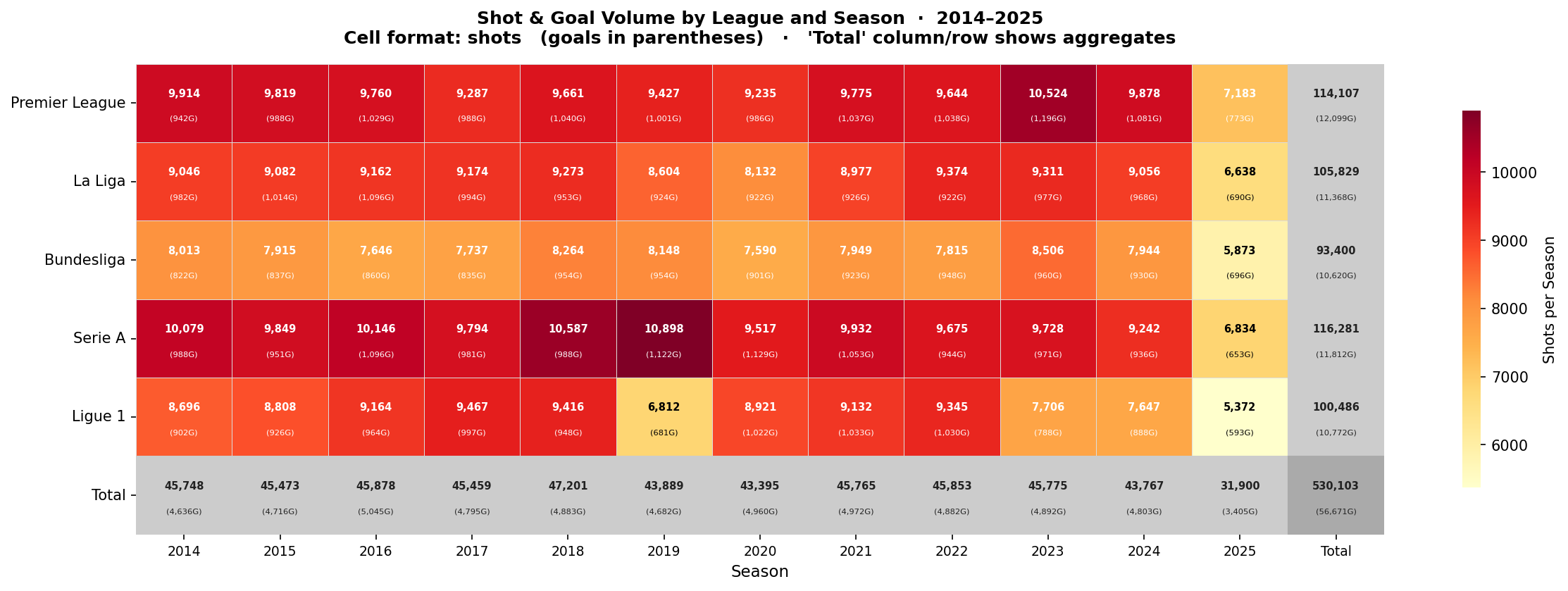
Figure: This dataset breakdown highlights the volume of shots and goals recorded across five major European leagues from 2014 to 2025. Compiling over half a million total shots is absolutely critical for training a robust classifier because actual goals are rare events (roughly one in ten shots results in a goal on average). The aggregated totals show consistent seasonal shot counts across the continent while providing a vast pool of positive historical examples for the model to learn from.

Cleansing

The cleansing stage is deliberately straightforward. It selects only the columns needed for modelling (X, Y, situation, shotType, result), coerces numeric types, ensures categoricals are consistent strings and drops anything malformed. Football shot data from a reputable provider is generally quite clean, and adding complexity here would be solving a problem that does not really exist.

Preprocessing and Feature Engineering

This is where things get more interesting. The raw coordinates are already normalised (values between 0 and 1, with the goal at x = 1, pitch centre at y = 0.5), so the coordinate features are usable directly. On top of those, two spatial features are calculated:

Distance to goal is the standard Euclidean distance from the shot location to the centre of the goal:

Angle to goal is computed using the dot product of the vectors from the shot location to each goalpost. This gives the angular width of the goal as seen from the shooting position, a more geometrically meaningful measure than a simple angle to the centre:

where \(\vec{v_1}\) and \(\vec{v_2}\) are the vectors to the two posts at \((1.0, 0.45)\) and \((1.0, 0.55)\) respectively.

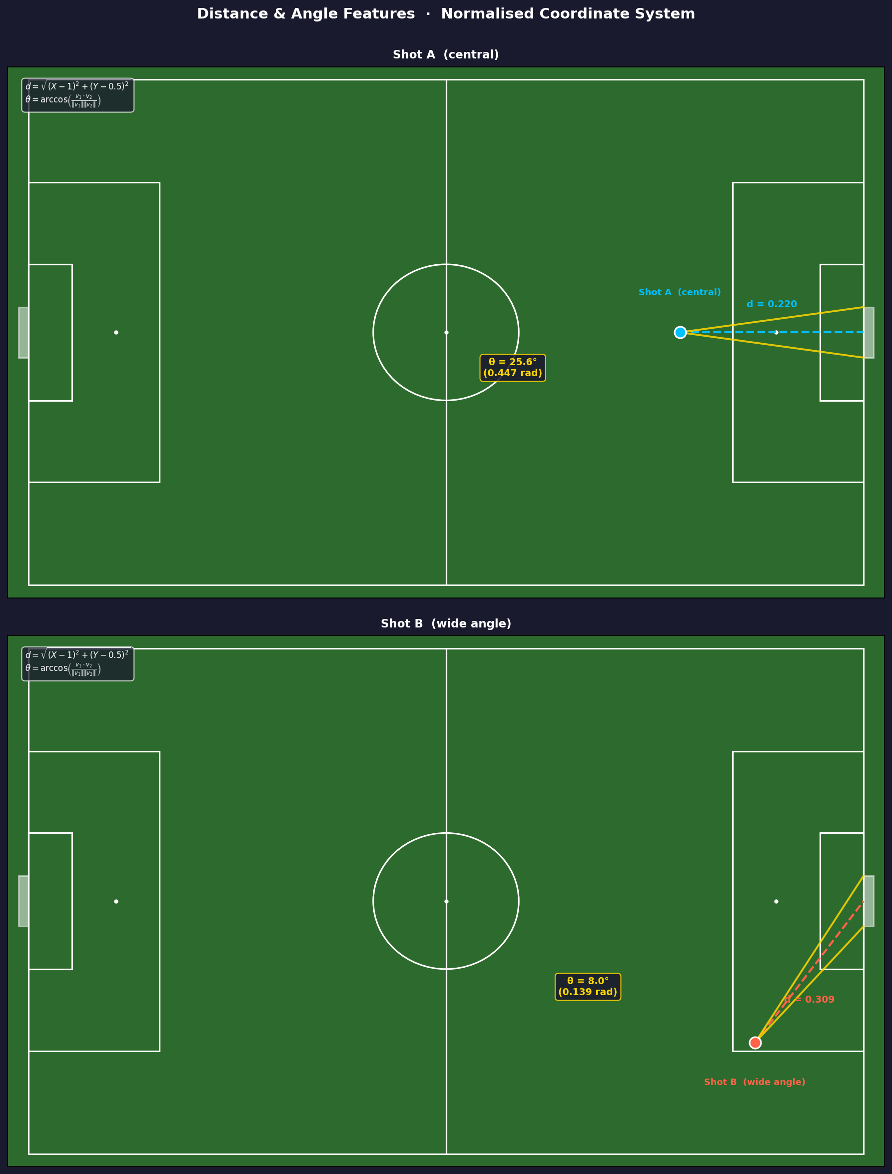
Figure: This schematic illustrates the two core spatial features underpinning the model. While distance to goal acts as a straightforward proxy for shot difficulty the angle calculation provides vital geometric context. A central strike and a wide attempt might share identical distances but the visible target area for the wide shot shrinks dramatically. Using this trigonometric approach ensures the algorithm understands goal face visibility rather than just raw proximity.

Categorical features (situation and shotType) are one-hot encoded using pd.get_dummies. The advanced model additionally includes interaction terms, created by concatenating the two category labels and then one-hot encoding the result, so OpenPlay_RightFoot, FromCorner_Head and so on become their own binary features. This allows the model to learn that, say, a headed shot from a corner carries different probabilistic weight than a right-footed shot from open play at the same coordinates.

The Model Architecture

Rather than a single monolithic model that handles all input combinations, the project trains four logistic regression classifiers, each suited to a different level of available information:

The Brier score measures the mean squared error between predicted probabilities and binary outcomes, so lower is better. To put the numbers in context, a perfect model scores 0. The scores here sit comfortably below 0.09, which suggests the models are doing genuinely useful work rather than producing elaborate shrugs. Each additional layer of information nudges them a little closer to the truth.

The reason for maintaining four separate models rather than one is straightforward. A user on the frontend may not always specify a shot type or situation, and imputing a value would be misleading. Instead, the system selects the most appropriate model at prediction time based on what information has been provided. No situation and no shot type? Use the basic model. Both provided? Use the advanced model. It is a clean solution and ensures the prediction is never artificially inflated or deflated by forcing a default category.

Training Details

Each model is trained using a scikit-learn Pipeline containing a StandardScaler followed by LogisticRegression. Hyperparameters are tuned with RandomizedSearchCV over 50 iterations, using 5-fold stratified cross-validation and Brier score as the optimisation objective. The search covers L1 and L2 regularisation with a log-uniform distribution over the regularisation strength C (spanning four orders of magnitude) and the liblinear and saga solvers.

With a large held-out test set of over 100,000 shots, the evaluation is on solid statistical footing. One of the lessons from the dissertation was that Brier score is a more informative metric than accuracy for a heavily imbalanced classification problem like this one. Goals represent roughly 10% of all shots, so a model that simply predicts "no goal" for everything would achieve 90% accuracy and be entirely useless.

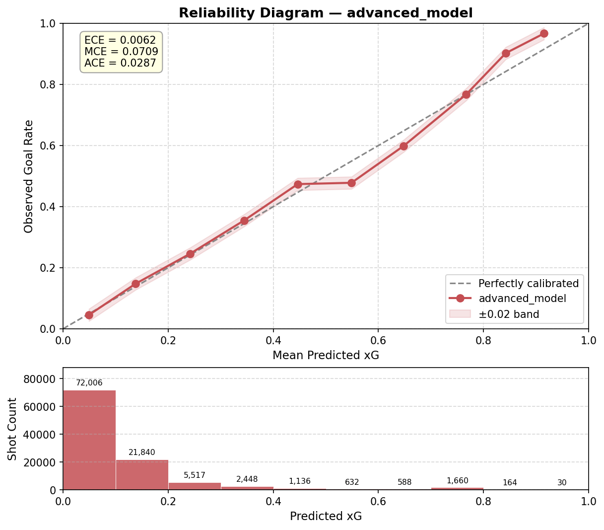
Figure: A reliability diagram visually assesses model calibration by plotting predicted probabilities against actual observed outcomes. The horizontal axis groups shots by their predicted expected goals value while the vertical axis shows the real percentage of those exact shots that resulted in a goal. If the model assigns a twenty percent chance of scoring to a specific batch of attempts a perfectly calibrated model will see exactly two in ten hit the back of the net. The incredibly low Expected Calibration Error (ECE) of 0.0062 and Absolute Calibration Error (ACE) of 0.0287 demonstrate that this model tracks closely to that ideal diagonal line across all probability buckets. The lower histogram highlights the severe class imbalance inherent to football data where goals are scarce and as such the model identified high-xg, clear-cut chances are few and far between.

Penalties are handled as a hard-coded override at prediction time, returning a fixed xG of 0.76 (the avg number of penalties scored for the dataset). Attempting to learn the penalty conversion rate from coordinates alone is rather circular when all penalties are taken from the same spot.

Transitioning from Flask to ONNX

The original version of the application used a Flask REST API to serve predictions. The frontend would fire a POST request on every click, the Python backend would run inference and return a JSON response. This worked fine locally but was a nightmare to deploy. It required a persistently running server, introduced latency on every prediction, and meant the project could not be hosted as a static site without paying for compute or fiddling with serverless functions.

The solution was to export the trained scikit-learn pipelines to ONNX format using skl2onnx and run inference directly in the browser via ONNX Runtime Web.

The export process (export_to_onnx.py) reads each model.joblib file, uses skl2onnx.convert_sklearn with FloatTensorType inputs and zipmap=False (to get a flat float32 probability tensor rather than a sequence of maps), and writes the resulting .onnx file alongside its metadata.json into frontend/models/. The heatmap data is copied across at the same time. After this step, the frontend directory is entirely self-contained.

In the browser, ONNX Runtime Web loads the models lazily and caches them, so the first prediction for a given model incurs a small network cost to fetch the .onnx file and every subsequent one is essentially instant. WebAssembly execution is fast enough that predictions feel synchronous from the user's perspective.

The xg_inference.js module is a JavaScript port of the Python inference logic, including coordinate normalisation, model selection, feature vector construction and the penalty override. The feature engineering, covering distance, angle and the one-hot encoding, is reimplemented in vanilla JS using exactly the same mathematical formulas as the Python preprocessing code. Any divergence between training-time and inference-time feature computation would silently corrupt the predictions, and debugging a model that is technically correct but fed subtly wrong features is not a particularly enjoyable afternoon.

The result is a web application that works offline after the initial page load, costs nothing to host beyond GitHub Pages, and makes predictions in the browser with zero network round-trips.

The Frontend

The frontend is built with HTML, Tailwind CSS and vanilla JavaScript, with no framework dependencies beyond ONNX Runtime Web. There are three pages:

Home (index.html) is an interactive pitch for single-shot predictions. Click anywhere, optionally set a situation and shot type, and the xG value updates immediately.

Heatmaps (heatmap.html) provides visualisations of pre-calculated xG values across the full pitch for each combination of situation and shot type. These are generated offline by generate_heatmaps.py, which sweeps a 100x100 grid of normalised coordinates at resolution 0.01 and stores the results in heatmaps.json. Pre-calculating rather than computing on the fly means the heatmap renders instantly and does not stress the browser.

Plotter (plotter.html) is the most involved page. It allows you to create a match with named home and away teams and custom team colours, plot shots for each side, and track the cumulative xG for both teams across the game. Shot data is persisted in IndexedDB so you can reload the page without losing your work.

The Pitch Canvas

The pitch is drawn on an HTML <canvas> element using FIFA standard dimensions (105m x 68m) with a 3m padding on all sides. All geometry is defined in metres and converted to pixels via a scale factor derived from the container width, so the pitch scales correctly to any screen size. Every pitch element (the goals, penalty areas, goal areas, centre circle, penalty spots, penalty arcs and corner arcs) is drawn programmatically from the FIFA Law 1 specifications. It is slightly more code than importing an SVG, but considerably more satisfying.

Shot markers are rendered as filled circles with a radius of 0.5 metres (scaled accordingly), coloured by team. The selected shot is highlighted with a ring. Clicking an existing shot selects it and clicking anywhere else plots a new one.

The Development Arc

The honest summary of how this project came together is roughly as follows:

1. The dissertation produced working Python models and a clear understanding of the feature space.
2. A Flask app was built to serve those models via an API, primarily as a learning exercise in building ML APIs.
3. The Flask app turned out to be awkward to deploy, which prompted the ONNX migration.
4. The ONNX migration opened up static hosting, which prompted building the match plotter as a more ambitious frontend feature.
5. The match plotter required IndexedDB, proper canvas rendering and a fair amount of JavaScript state management, all of which was built from scratch.

The dissertation is where the model design and much of the analytical thinking lived. The plotter is where the engineering happened. The two fed into each other more than a numbered list makes it sound.

What I Would Do Differently

A few things stand out with the benefit of hindsight.

The four-model selector is clean from a user experience perspective, but it adds meaningful complexity to the JavaScript inference module, which has to maintain feature lists in sync with the Python training code. A single model trained on all features, with a learned imputation or embedding for missing categoricals, would simplify the inference path at the cost of some interpretability.

The data covers the top five European leagues from 2014 to 2025, which is broad but not necessarily deep. A model trained purely on shot coordinates and categorical context will always be limited. It has no knowledge of the defensive pressure on the shooter, the quality of the assist, whether it was a first touch or a controlled finish, or any of the richer context that commercially developed xG models incorporate. For a personal project this is entirely fine, though it is worth being honest about the limitations if anything more serious were on the table.

Tech Stack Summary

• Data and modelling: Python, pandas, scikit-learn, NumPy, skl2onnx
• Model format: ONNX (via skl2onnx export from scikit-learn pipelines)
• Frontend: HTML, Tailwind CSS, vanilla JavaScript, ONNX Runtime Web
• Persistence: Browser IndexedDB
• Hosting: GitHub Pages (fully static)